Visualising discrete wavelet transforms: updated for RapidMiner v8

I revisited a previous post about visualising discrete wavelet transforms because I wanted to remember how I did something. The process is quite old and did not work first time with version 8 of RapidMiner Studio. There have been some subtle changes with respect to the requirements for the type of attributes for the "Join" and "De-Pivot" operators. Never fear, I've updated the process and it's here.

Here is the money shot to prove it still works

An interesting feature of this process is the way it uses the "De-Pivot" operator to transform a matrix-like example set into x,y,z coordinates that can be plotted.

Processing value series

Value series are tricky to get working and in fact, there are some operators that I just can't make work.This is not the end of the world but to save head scratching time, here is some explanation and a process that captures the essential features of value series for reference purposes. The process finds the frequencies contained in some artificial data in two ways using value series techniques and in so doing, the results can be checked against one another to give insight into how value series work.

The first thing to say is that there are two types of value series operator. One type works on example sets, the other on example sets that have been transformed into series.

The first type is contained in the sub group "Data Transformation" and includes operators like "Differentiate" and "Integrate". These require an example set and require one attribute to be selected for processing. The operators assume the examples in the example set are an ordered time series and the attributes represent how data varies as a function of the examples.

The second type - the subject of this post - includes operators in the "Series Transformation" group. Here, the operators require a series object and these are produced using the "Process Series" operator or the "Data To Series" operator. This latter operator works in two ways; either by treating the attributes in an example as members of the series ("series_from_attributes"), or by using one particular attribute as the series variable with the ordering dictated by the example set ("series_from_examples").

One important point in the "series_from_attributes" mode is that only a single example within an example set can contribute to the series. This means that filtering of examples must happen in order to produce a series and this must happen in a loop to perform the processing on each example.

Putting all this together, the following picture shows the top level view of a process that uses both the "Process Series" and "Data To Series" operators.

The generated data is a superposition of three random sine waves with random amplitudes. The top branch shown below performs a Fourier analysis on the data and uses the "Extract Peak" operator to find the maxima of the frequency spectrum. The "Process Series" operator uses the attributes in a single example to generate the series to pass to the inner operators. In effect, this operator is iterating over all the examples in an example set.

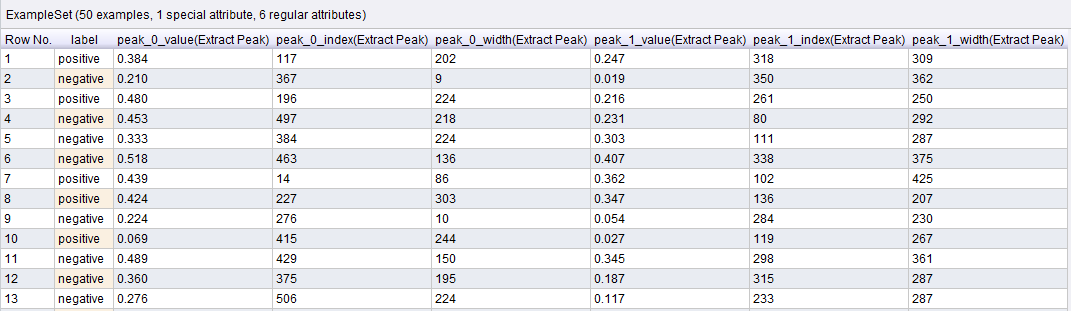
The resulting example set looks like this

As can be seen, example 1 has a maximum at 117 and a secondary peak at 318. Example 2 has a maximum at 367 and another at 350 and so on.

The lower branch processes the data using a different series approach. The picture below shows the inner operators within the "Loop Examples" operator.

The output from one iteration of the loop is fed back to the next iteration and to make this work requires the example set to be passed straight through via the "Multiply" operator. The second output is generated by the following steps

• Filter for the single example
• Convert to series using "series_from_attributes"
• Calculate the Fourier transform
• Convert back to an example set
• Add an attribute to show the example being processed

The output is a collection which can be combined into a single example set using the "Append" operator and following a bit of light pivoting gymnastics, graphs can be drawn of the Fourier transforms for each of the examples.

Shown below are the graphs for the first (red) and second (blue) examples. As can be seen, the peaks match what was calculated above.

In real life, you would probably not use both approaches in the same process. The "Process Series" operator is generally easier to use since it acts as a shortcut but if your data is encoded as examples then you either have to use the "Data To Series" approach or do some windowing to convert adjacent examples into attributes.

Visualizing discrete wavelet transforms: part II

Here is a process that takes the discrete wavelet transform (it happens to be the Daubechies 4 wavelet in this case rather than the Haar but the results are similar) of some fake data and plots the corresponding results. This is different from the maximum overlap discrete wavelet transform from the previous post.

The result looks like this.

(the z2 attribute is plotted as the colour using log scaling)

The bottom row is the clean signal (with scaling to make it show up), the 2nd row from the bottom is the noisy signal and the third row from the bottom is the result of the discrete wavelet transform. This is only included for completeness since it does not correspond in the original domain to the signal. For an interpretation of this I found the following in the code of the discrete wavelet transform (in file DiscreteWaveletTransformation.java)

In the case of the "normal" DWT the output value series has just one dimension, and these
coefficients are to be interpreted as follows: the first N/2 coefficients are the wavelet
coefficients of scale 1, the following N/4 coefficients of scale 2, the next N/8 of scale
4 etc. (dyadic subsampling of both the time and scale dimension). The last remaining
coefficient is the last scaling coefficient.
 
So this means the 4th row from the bottom corresponds to the coefficients of scale 1, the 5th row to scale 2 and so on. The coefficients have been replicated as many times as required to match the x scale.
 
Note that this differs from the view tradionally presented in the literature where the high frequencies are presented at the top. That's an exercise for another day.
 
The main difference between this and the previous MODWT example is the unpacking of the DWT result. For this I used a Groovy script. This takes 2 example sets as input and copies the correct parts of the first (the DWT result) into the second (the output that will eventually be de-pivoted).

The output example set that is fed into the Groovy script is created using a "Generate Data" operator since I found this to be the easiest way to generate the example set with the right number of rows and columns.
 
As before, the graphic shows that the algorithm has seen the presence of the low frequency signal at the expected location from x = 5000 and there is perhaps a hint that something has been spotted at x = 100.

Visualizing discrete wavelet transforms

RapidMiner can transform data using wavelet transforms within the value series extension. As part of my endeavour to learn about these I made a process that allows visualisation of the results of a MODWT transform. It's intended to show at a glance what the transformation has done to the data.

Amongst others, it uses the "data to series", "series to data" and "de-pivot" operators and of course the "discrete wavelet transform".

The process creates some fake data consisting of 8192 records. A high frequency square wave is located from position 100 to 600 and a lower frequency wave is located from 5000 to 5500. A significant amount of noise is also added to hide the signal.

If you plot the results of the de-pivot operation and use the block plotter, choose x, y and z2 and set the z2 axis to a log scale, you should see something like this.

The bottom row corresponds to the pure signal (note its amplitude has been scaled to make it show up better), the next row up the noisy signal and all the rows above that correspond to the different output resolutions of the MODWT transform. The top row is the average for all the signals and should be 0 owing to the normalisations performed on the input data. All of this is produced from the MODWT output using the de-pivot operator after a certain amount of joining gymnastics.

The plot shows that the transform has detected a match from the 5000 point for the original signal. The signal from 100 is not so obvious.

The individual outputs from the MODWT operation are also available. Here for example is a plot of the 6th output (i.e. the 8th row in the graphic above).

Compare this with the raw noisy data.

Clearly there is something in the data and the transform is able to isolate this to a certain extent.

My next process will be one to visualise the DWT rather than the MODWT output.

Differentiate value series

Copy of the process from my posting from the Rapid-I forum

Link to file

Still works in version 5.1

Value series example

Copied from my posting on the Rapid-I site

Link to file

(Still works with 5.1)

(Still works with 5.2)

Fast Fourier Transform Example

Originally posted by me (awc) on the neuralmarkettrends forum

See file here

Note: later update to fix a bug in 5.1 where attribute names cannot be reserved words

Note2: the data is available on the neuralmarkettrends forum posting and is also here

Using NullGenerator in value series preprocessing

Here's an example that uses value series preprocessing (This no longer works in 5.1 - the series operators have not worked well in version 5 as a whole)

<operator name="Root" class="Process" expanded="yes">
<parameter key="random_seed" value="-1"/>
<operator name="GenerateSeriesIOObjects" class="OperatorChain" expanded="no">
<operator name="Generate a sine wave SeriesIOObject" class="SinusGenerator">
<parameter key="number_of_values" value="2000"/>
<list key="frequency">
<parameter key="101" value="1.0"/>
</list>
</operator>
<operator name="Visualizer (2)" class="Visualizer" activated="no">
</operator>
<operator name="Convert into an ExampleSet" class="SeriesObject2ExampleSet">
</operator>
<operator name="Window into examples" class="MultivariateSeries2WindowExamples">
<parameter key="window_size" value="1002"/>
</operator>
<operator name="Add a label" class="WindowExamples2ModelingData">
<parameter key="label_name_stem" value="sinus_dim_1"/>
<parameter key="relative_transformation" value="false"/>
</operator>
<operator name="Delete the Id" class="AttributeFilter">
<parameter key="condition_class" value="attribute_name_filter"/>
<parameter key="parameter_string" value="sinus_index"/>
<parameter key="invert_filter" value="true"/>
<parameter key="apply_on_special" value="true"/>
</operator>
<operator name="Add an easier to read Id" class="IdTagging">
</operator>
<operator name="Change examples into seriesIO objects" class="Single2Series">
</operator>
</operator>
<operator name="ValueSeriesPreprocessing" class="ValueSeriesPreprocessing" expanded="yes">
<operator name="Branch" class="Branching" expanded="yes">
<parameter key="keep_only_last" value="false"/>
<operator name="Find the maximum frequency within each window" class="OperatorChain" expanded="yes">
<operator name="Split each example into 5 windows" class="Windowing" expanded="yes">
<parameter key="step_size" value="200"/>
<parameter key="window_size" value="200"/>
<operator name="OperatorChain (4)" class="OperatorChain" expanded="yes">
<operator name="DiscreteFourierTransform (2)" class="DiscreteFourierTransform">
</operator>
<operator name="MaxIndex" class="MaxIndex">
</operator>
</operator>
</operator>
<operator name="NullGenerator (4)" class="NullGenerator">
</operator>
</operator>
</operator>
</operator>
</operator>

This process does the following things

1. Generates a set of examples each containing 1001 attributes
2. Each example is converted into a SeriesIO object
3. Each SeriesIO object is split into 5 windows each containing 200 values
4. A Fourier transform is performed on each window and the index where the maximum is located is found
5. The NullGenerator operator causes the maximum index for each window to be returned. This has the effect of returning the maxima for all the windows.